Generalized version of Two Envelopes problem
Variants vG, vD, vS, vA, vN …
Resolution of paradox
Expected values and paradox
Infinite Expected values
Expected gain and paradox
Optimal strategy if we can look into envelope
Solution of Generalized version ( answer to Q1 )
Optimal solution of Generalized version (answer to Q2)
vD: default variant where player select envelope
vS: standard default variant where second envelope is doubled
vX: standard variant where we directly choose value X
vU: simple uniform variant
vUc: continuous uniform variant
vA: ‘always better’
 variant
vAc: continuous ‘always better’ variant
vN: Nalebuff asymmetric variant
Summary
Problem definition
Standard version of this paradox, to quote Wikipedia, is :
Imagine you are given two identical envelopes, each containing money. One contains twice as much as the other. You may pick one envelope and keep the money it contains. Having chosen an envelope at will, but before inspecting it, you are given the chance to switch envelopes. Should you switch?
Further description of steps that lead to apparent paradox:
- Denote by A the amount in the player’s selected envelope.
- The probability that A is the smaller amount is 1/2, and that it is the larger amount is also 1/2.
- The other envelope may contain either 2A or A/2.
- If A is the smaller amount, then the other envelope contains 2A.
- If A is the larger amount, then the other envelope contains A/2.
- Thus the other envelope contains 2A with probability 1/2 and A/2 with probability 1/2.
- So the expected value of the money in the other envelope is :

- This is greater than A so, on average, the person reasons that they stand to gain by swapping.
- After the switch, denote that content by B and reason in exactly the same manner as above.
- The person concludes that the most rational thing to do is to swap back again.
- The person will thus end up swapping envelopes indefinitely.
- As it is more rational to just open an envelope than to swap indefinitely, the player arrives at a contradiction.
That is basic and fairly generic definition of the paradox. But, while it does not define how is money selected for envelopes, it does specify that initial envelope is picked at random – which exclude certain variants of Two Envelopes problem like Nalebuff variant ( where specific envelope is given to player ).
Generalized version of Two Envelopes problem
It is possible to generalize problem so that it covers practically all variants than can be called “Two Envelopes paradox”. Assume we have host who choses values in envelopes, and player who gets envelope and chooses to switch or not:
- host randomly select value R with p1(r) probability distribution
- host puts X=V(R) amount into first envelope
- host puts double amount in second envelope (2X) with probability D, otherwise puts half (X/2)
- player is given or select first envelope with probability F, otherwise player gets second envelope
Q1) without looking in envelope, should player switch to other envelope ?
Q2) with looking in envelope, when should player switch to maximize gain ?
Each variant of Two Envelopes problem can be defined with these four parameters: p1(r), V(r), D, F. Question Q1 is one that supposedly lead to paradox in original variant, while Q2 is optional question about optimal strategy to maximize gains.
First parameter is probability distribution p1(r) that determine how probable is intermediate value R that is then used in ‘value’ function V(R) to get X amount which goes into first envelope. For continuous values of X, R has continuous probability distribution and p1(r) is proper probability density function such that  . If R has discrete probability distribution then p1(r) is proper probability mass function such that
  .
.
Generic problem is using intermediate random variable R and its associated probability distribution  instead of directly generating value X using probability distribution
  due to several reasons:
- to be able to cover with generic problem those variants like vA that state “randomly select R and then put
 into first envelope”
 - to cover variants that have proper probability distribution for R even if they have improper distribution for X
- to cover variants that use continuous distributions to generate discrete values, like
 and
and 
Both parameters F and D are probability values and so in range 0..1, assumed constant for given variant (even when unspecified, like in original variant ). Default Two Envelopes problem states that  , and does not specify D ( paradox claims remain same, regardless if host double or half value in second envelope ). But some modified variants ( like Nalebuff ) use different F ( F=1, host always give first envelope to player) and specify D (D=
 , to ensure
  outcome if switching ).
It is possible to even more generalize Two Envelopes problem, by making even probability for host to double value in second envelope and probability for player to get first envelope as functions of R, meaning not only V(r) but also D(r) and F(r). While this would make it harder to find general solution (there is one presented below), it would make it even harder to create meaningful problem variant that would have visible paradox – since paradox need believable claim of type “so for every value of X it is better to switch”, and it is hard to make that claim obvious if benefits of switching change with each value.
Variants vG, vD, vS, vA, vN …
Variants of “Two Envelopes” problem differ in what and how they define one of four parameters in generalized definition of problem. Variants are named as ‘vX’, to be easier to refer to them in text, but it should be noted that some of those variants are actually sub-variants of other more generic ones ( eg. vA is subvariant of vS which is subvariant of vD), with all of them being sub-variants of most generic vG :
- vG (Generic) : all four parameters F, D, V(R) and p1(R) are unspecified ( and thus any valid)
- vD (Default, F= ): player select envelope so F
 while D, V(R) and are unspecified
- vS (Standard, D=1): F , D=1 while V(R) and are any
- vX (Direct standard, X=V(R)=R ): F , D=1, X=V(R)=R , while
 is any
- vU (uniform discrete): F , D=1 , V(R)=R, p1(R)=
 for
for 
- vUc (uniform continuous): F , D=1 , V(r)=r, p1(r)= for
![r \in [0,N]](https://gmnenad.com/wp-content/ql-cache/quicklatex.com-8c44d7ead8936a937d65f75c1a916dba_l3.png "Rendered by QuickLaTeX.com")
- vU (uniform discrete): F
- vB (Binary, V(R)=): F , D=1 , V
 , while is any
- vA (discrete ‘always better’) F , D=1 , V , p1(R)=

- vAc (continuous ‘always better’) F , D=1 , V , p1(r)=

- vA (discrete ‘always better’) F
- vX (Direct standard, X=V(R)=R ): F
- vS (Standard, D=1): F
- vN (Nalebuff): F=1 , D , while p1(R) and V(R) are unspecified/any
- vD (Default, F=
For Default variant vD and all of its subvariants it is proven below that formulas for their expected values when always switching are same as expected values when never switching ( ) and thus paradox does not exist. Formulas are also derived for expected values if switching when value inside envelope is less than some value H,
  , and for finding optimal value
  that maximize
  .
.
For Nalebuff asymmetric variant vN it is shown that it indeed has better expected value if switching, but that it is not same if again switching back – as it’s name suggest, it is ‘asymmetric’ and same reasoning can not be applied for other envelope after switch.
Resolution of paradox
There are many proposed resolutions of this paradox. Most of them focus on step #6 from 12 steps – stating that it is impossible to put money in envelopes in such a way that for any possible value in selected envelope other envelope has equal chance of containing double or half.
Simple example would be if we randomly with equal chance select for first envelope out of 2,3,4 and put double in second envelope. It is easy to see that claims from above paradox are valid only if you have 4 in your envelope – only then other envelope has equal 1/2 chance of being double (8) or half (2), and only then your expected value if you switch would be 5/4x. But consider case when you have 1 or 3 in your envelope – there is 100% chance that it is smaller value, not claimed 1/2, and it give you even larger 2x if you switch. On the other hand, when you have 6 or 8 in your envelope there is 0% chance that other envelope has double that value, and switching would clearly result in loss with expected x/2. It can be shown that all possible gains in switching on smaller values 1,2 or 4 are exactly offset by losses if switching on larger 6 or 8.
In fact, in almost all variants paradox does not exist due to one of these two claims being false:
#2) equal chance other is smaller/larger: the probability that A is the smaller amount is 1/2, and that it is the larger amount is also 1/2 ( for any possible value in envelope )
#9) indistinguishable envelopes: after the switch, denote that content by B and reason in exactly the same manner as above
But for almost any proposed resolution some counterexample was proposed, by either slightly modifying problem setup or how money is selected for envelopes, that counter suggested resolution. Examples of such modified problems are Nalebuff variant that guarantee #2 for first envelope, or  variant where it appears that it is always best to switch.
Expected values and paradox
Paradox can be resolved by pointing to each separate false claim, but it can also be resolved by calculating expected value if we would never switch envelope ( ) and showing that it is same as expected value if we always switch envelope (
 ). Expected value can be described as an average value that would be earned if this game is played many times. Thus it is product of amount of money in selected envelope and probability for that amount to appears.
To really prove that there is no paradox, it is not enough to just calculate expected values for one specific case – we need to find formulas for expected values and show that they are identical when switching or not switching.
We can use several different approaches to find formulas for expected value, and they notably differ in selecting random variable over which we would sum or integrate: over values of first envelope ( ‘first’ is one where host first puts money as defined in generalized problem ) or over values in envelope that player gets/select or over possible values for random number generated before we determine value for first envelope etc. Other difference is whether probability is continuous or discrete, which determine whether we sum or integrate over all possible probabilities. To demonstrate those different approaches, we will simplify and consider here only subset of generalized problem where V(r)=R ( but solution for fully generalized problem is given in later section, using one of approaches demonstrated here ). This means subvariant where we directly generate random value X for first envelope (so  instead of
  ), and we always double second envelope ( so first one is always smaller).
First approach to find expected value when we never switch () is going over all possible values in smaller envelope, and  is probability to put X as value in smaller envelope, while
  is probability that player will get envelope with smaller value (
  when player select randomly one envelope ):
 ( condition for valid selection of values)


Second approach is instead going over all possible values in selected envelope, and  is probability for player to select/get envelope with value X:
 ( condition for valid selection of values)

Both approaches are also applicable when probability to put values in envelopes is not discrete but continuous ( which is arguably more generic approach, since continuous probability selection can be extended to cover discrete ones) . In this case  is continuous probability density function for putting value in smaller envelope:


And accordingly if we use  as continuous probability density function to have value X in envelope we select/get:


Finding expected value if we always switch () is done in the same way, just swapping sides for smaller and larger payoff, while  is probability that player will get envelope with smaller value ( which in this case depends on X, and is different than ). So:

 , or
, or
 , or
, or
 , or
, or

Some variants of Two Envelopes problem can separate probability distribution and value in envelope, by first selecting random R with some proper probability distribution  , and then put V(R) in envelope ( function based on R, instead of just putting R in envelope) and then double that value for second envelope. Previous approach of directly selecting X is subset of this one, when X=V(R)=R. We can modify formulas for expected values for those variants:


For default Two Envelopes variants, where player is allowed to select envelope, we always have  , so :


Therefore for all standard variants expected value if switching is equivalent to expected value when not switching ( ) , regardless of way in which money is put in envelopes . That means it is same if you switch envelopes or not, which resolves paradox.
Infinite Expected values
In some cases expected values may be infinite, even with valid probability distributions. One example is vA variant discussed later, where  and
and  . When those variants have player selecting envelope, their expected values when switching or not switching will still be same as demonstrated above – same as in ‘same formula’, but they would be infinite values.
Some people would say that we can not compare two infinite expected values and state that they are ‘same’, and thus we can not use them to resolve paradox. Other people would say that variants with infinite expected values are invalid (there is not enough money in the world), so there is no need to resolve them.
Both of those positions are actually wrong. Second position is easier to disprove – since variants like vA are doable in reality (just write amounts on cheque instead of putting actual money, and it is irrelevant if you can not draw on that cheque), we can not ignore them. First position is harder to disprove but it rely on fact that we do not need to directly ‘compare’ expected values, we just need to prove that they are indistinguishable – in which case it would not matter if we switch or not, again resolving paradox.
In this case, we want to prove that when we have expected values with same formulas for both switching and not switching, even when those expected values are infinite they are indistinguishable and thus it is same if we switch or not .
One way to prove it is to imagine two players playing game many times in parallel: A will always chose not to switch in his game and B will always chose to switch in his game. Can we distinguish those two players just by their total earned amount when they exit after same (possibly very large) number of games ?
When game has identical formula for expected values when switching or not, we would not be able to tell which was player A and which was player B even if expected value was infinite. While with infinite expected value their total earned amount could be significantly different even after millions of games, we would not be able to say which one was lucky enough this time to get that rare very high value in one of their envelopes. In other words, players A and B have equal chance to exit with higher amount, and equal chance for how more/less they could have compared to other player.
This makes them indistinguishable, thus proving out point that it is same if they switch or not. This same principle holds regardless if expected values were infinite or not, with only difference than non-infinite expected values would tend to result in very similar total earned money for both players. Note that we have even higher order of ‘indistinguishability’ that we really need : we only needed total expected values to be indistinguishable, but that could be result even when formulas for expected values are different but total sum result in same expected value. But when we have same formulas for expected values we also have same probability for any individual value in envelopes. In other words, we could not distinguish between players A or B even if we can see amount they earn after each individual game. For infinite expected values that means we will see they both have almost exact same frequency of lower values (that appear more often), and would potentially differ in those much rarer very high values.
Above claims would be harder to prove if formulas were infinite sums involving both positive and negative signs – like for example in expected expected gains. In those cases results of sums would not only be converging to some finite value or diverging to infinity ( but with same ‘indistinguishable’ behavior as described here). Infinite sums with alternating signs can also result in undefined finite value – value that would periodically change as each new element is added to sum. Those sums could apparently have different result values depending on how we rearrange elements, but it is only ‘apparent’ value – actual result of such sum is ‘undefined’. If two values would have same formula with such undefined sums we could still argue that they are indistinguishable and could be compared, but if such sum is single result as in expected expected gain case we could not prove validity of such sum in infinite case. But for expected values used here, sums or integrals always involve positive values, so there is no ambiguity.
Another way to prove that infinite expected values are comparable is to imagine three players, each doing single game : A will chose to not switch while B and C will chose to switch. But before they open their envelopes, player C can chose to swap his envelope with either player A or B, or to keep his own. Can he expect better value if he swap with B or if he keeps his own envelope? What about A?
Depending on your position regarding “we can compare infinite expected values”, your answers to “Can he expect better value if he swap with B or if he keeps his own envelope?” can be:
- ‘no’ : he can not expect better value if he swap with B ( for example because they both played in exactly same way – both were switching ). But regardless of why you chose to say ‘no’, it means that you are able to ‘compare’ those two cases even when their expected values are infinite – and thus same logic can be applied to A, with conclusion that they are indistinguishable
- ‘undefined’ : if you think we are unable to compare infinite expected values, we can not say if C or B can expect better. But that makes choice of B indistinguishable from choice of A, making again switching or not switching indistinguishable
- ‘yes’ : probably no one will chose this answer. It could be proven that it is invalid answer but, regardless of reason behind it, it follows same logic as ‘no’ – it means you accept ability to compare infinite expected values. So we can just claim that two same expected formulas are ‘same’ even with infinite value, again making switching or not switching indistinguishable
Yet another approach is to establish even higher order of ‘comparability’ between two expected value formulas that both has infinite value – not just if they are indistinguishable, but to actually compare ‘how many times is one better than the other’ . Assume we select random value  ( n=0,1, … ) with probability , and put
  in first envelope. Then we select another value (
 ) with same probability distribution and put this time
  in second envelope. Which envelope you should select?
In this case values in two envelopes do not depend on each other and envelopes will even contain different possible numbers ( eg second envelope can have 3, but can not have 4 ). Also, both envelopes have infinite expected value but it is clear that if first envelope has expected value  , second envelope has triple that value, or
  .
.
Even those subscribing to ‘we can not compare infinite expected value’ would be hard pressed here not to state that it is always better to select second envelope. In fact, we could say that selecting second envelope should on average result in triple gain. In other words, if relative ratio of expected values is valid number, it should be valid even if expected values were infinite. In this case  . And we should switch only if
  , which in this case is true. Applied to our general formula for any Two Envelope problem where player can select envelope:
 does not matter if we switch
Thus we proved that when expected values for switching and not switching have same formula, even if those result in infinite values, it is indistinguishable if we switch or not – therefore avoiding paradox. And since we previously proved that expected values for switching and not switching always have same formula and values if player can chose envelope, this resolve paradox for all standard Two Envelope variants.
We could drive this logic even further and say that , regardless if expected values are same for switching or not switching and regardless of infinity of expected values or even invalidity of probability distributions, we can either distinguish between player who always switch and one who never switch or we can not, based just on their total earning. If we can distinguish, we should chose to do whatever one with better total earning is doing – and there is no paradox, since we should not ‘chose back’ else we would get lower value. If we can not distinguish between them, then it is same if we switch or not – again resolving paradox.
Expected gain and paradox
Alternative way to resolve paradox is to show that there is no gain if switching. In other words, showing that difference between expected value when switching and not switching is zero. Simple formula for expected gain would be:
If  there is no paradox
While this simple formula is easy to understand, it has certain disadvantages : it still require finding separate formulas for and and it is not very informative ( unlike formulas for and which can tell players what to expect after game ). But, most importantly, it is hard to prove validity of this approach if those expected values are infinite. We can claim resolution of paradox even in case of infinite expected values when comparing two values with identical formulas – we only need to accept that values derived with identical formulas are identical and indistinguishable even if infinite. But claiming that subtracting those infinite values result in zero could be considered as additional “extension” of infinite arithmetic, especially since we can not use ‘indistinguishability’ to prove it.
There is better approach : expected expected gain (EEG). Instead of gain as difference between total expected values, for each possible value in selected envelope determine expected gain as difference between expected value if switching vs not switching only for that value in envelope. That would be ‘expected gain’ for that specific value in envelope, but since values in envelope do not all have same chance to appear, total gain would be sum of those individual expected gains multiplied by probabilities of each value. In other words, expected value of expected gains , and thus double ‘expected’ in name ‘expected expected gain’, or EEG for short.
While finding value for such expected expected gain would still be less informative to players than expected values, it could avoid other two disadvantages : it does not need calculating and , and in some cases it could avoid infinite results. Just like expected values, finding formulas for EEG could use sum/integral over different probability distributions: p1(r) for generated value in ‘first’ envelope, or probability of values selected by player etc. In any case, proving resolution of paradox would in this case be:
If  there is no paradox
But proving above is still more problematic than proving , especially for only case where ‘paradox’ can still remain: infinite expected values. It is theoretically possible that for some specific variants we could have finite EEG even with infinite expected values. But since such EEG would involve sums ( or integrals ) of individual expected values, that means infinite sums of alternating positive and negative signs – and it is known that such infinite sums can result in ‘undefined’ values : apparent different finite results, depending on how we rearrange elements in sum.
When proof depends on comparing two entities with same formulas but possible infinite values ( like comparing to ) , we can claim that since those values are indistinguishable they must be considered ‘same’ – and it would maybe hold as line of reasoning even for undefined sums with alternating signs ( regardless how you decide to rearrange that sum, when done to both entities it would result in same values ). But it can not be done for single entity – proof of EEG claim is not comparing EEG formula to some other EEG formula, but to zero. And we can not claim that such undefined EEG is ‘undistinguishable’ from zero – depending on how we decide to calculate/rearrange such EEG sum, it will result in different values while zero will always be zero.
Bottom line is that EEG with infinite sum ( due to alternating signs) is not valid method to either prove or disprove existence of paradox. Because of that, expected gains ( or expected expected gains ) are not used in this document to prove resolution of the paradox – all proofs are based on formulas for expected values, which even for infinite cases are sums/integrals for always positive values which either converge to same finite value or diverge to infinity in ‘same’, undistinguishable way.
Optimal strategy if we can look into envelope
Finding and and showing that they are same is enough to resolve paradox, as they will show that it is same if we always swap or never swap – which are only options that we have if we can not look into envelope that we got before deciding whether to switch or not.
But if we are allowed to look into envelope, it is possible to make more informed decision on switching, which should yield optimal expected value  which is better that and . General approach to optimal strategy is to switch if we see smaller value in envelope and do not switch if we see larger value in envelope. Obviously, “larger” or “smaller” will depend on probability distribution when selecting value for envelopes, but in any case it means that optimal strategy would require finding optimal H so that :
If value in envelope is  , switch when
Above is not only better but also optimal approach when probability and value functions are monotonous. We can define expected value if we switch on H, which is calculated similar to and , by switching before H and keeping after H. Assuming is probability to get X in your selected envelope, and  is probability that X is smaller of two values, then formula for
  , by integrating over possible selected values in envelope, is :
![E_h(H)= \int\limits_{x=0}^{H} p_{sx}(x) \cdot [p_{smaller}(x) \cdot 2x+p_{larger}(x) \cdot \frac{x}{2}] dx + \int\limits_{x=H}^{\infty} p_{sx}(x) \cdot x \;dx](https://gmnenad.com/wp-content/ql-cache/quicklatex.com-6f477bd799192c11aca65648e09ffc8b_l3.png "Rendered by QuickLaTeX.com")
Extreme values for H are zero and infinity, and they correspond to never switching and always switching:


In default Two Envelope variants, where player can select envelope, will rise from with increasing H up to some when expected value will be  , after which it will fall back toward as H goes to infinity.
Actual optimal value H depends on specific parameters of problem, like probability distribution. But since any H between zero and infinity can only increase expected value when compared to always switching or always not switching, rule of thumb approach ( when not knowing specific random distribution parameters, but participating in multiple choices ) would be to switch if X is smaller than half of largest seen value so far. If participating only in single choice, approximate optimal strategy without knowing parameters would be:
Switch if value in opened envelope is smaller than half of whatever you guess could be maximal value in envelopes.
Solution of Generalized version ( answer to Q1 )
Most variants of Two Envelope problem ‘fail’ at either not satisfying #2 claim ( for any possible value X in selected, probability that X is the smaller amount is 1/2, and that it is the larger amount is also 1/2 ) or not satisfying #9 claim ( after the switch reason in exactly the same manner as before, and conclude to switch again ).
But instead of specifically pointing out different failings of different variants, generic approach would be to disprove one of two common claims that they all have:
c1) Even without looking in first envelope, it is better to switch to other envelope
c2) After you switch to second envelope, same reasoning can be applied and you should switch again
Different variants arrive at those claims by different approaches but they all end with those, leading to apparent ‘paradox’.
First claim would be valid if expected value when player switch () is larger than expected value when player does not switch (). Therefore it is enough to either find formulas for those two expected values and show that , or calculate actual expected values when possible and show that  .
.
Expected value when player does not switch can be calculated in different ways, but probably easiest is to calculate over every possible value R ( and corresponding value X ) in first envelope. For discrete probabilities that would be:

Where  is value in first envelope (one where host first put money, not one that player necessary took) and
  is value in second envelope ( which will be 2*first if doubled or first/2 if halved):

When we replace F= and
and  , we get:


It is exactly same approach for expected value when not switching with continuous probabilities, only using integration instead of sum:


Expected value when switching is calculated in similar way, only value in second envelope is used when first envelope was given ( and vice versa):


And again same approach for expected value when switching with continuous probabilities:


As it can be seen, expected values when switching or not switching have almost same formula, sums/integration over same range with only difference in constant coefficient influenced by F and D parameters. We can denote as Z that common sum/integrate part:
 , for discrete distributions or
 , for continuous distributions


When we compare those two expected values, we can see that they are not necessarily always same, thus leaving some room for paradox. Condition for those two to be same ( and thus eliminate paradox, since it would be same if switching or not switching) is :


We use  symbol to denote ‘equivalency’ of two formulas, meaning that they are ‘exactly’ same : not only their values are same but they are calculated in the same way, over same integral/sum ranges, and thus comparable ‘same’ even when calculated value is infinite. Notably, for all variants of Two Envelopes problem that follow original setup and have player picking up one envelope, we have
  and thus:

That means expected values when switching or not switching are always same if we let player choose envelopes or in any other variant where host give first envelope with chance. Therefore in all of those variants paradox is resolved – it is same if you switch or keep envelope.
There are some variants that do not have , like Nalebuff vN variant. In that particular case we have F=1,  , and thus:
 but
but 
Therefore if you switch you can expect  more value even without looking in envelope. But Nalebuff variant fails to be paradox due to step #9, since same reasoning can not be applied to second envelope – envelopes are not indistinguishable. In fact, if you switch back, you can now expect just Z, or less than what you could expect if you stayed with second envelope.
In general, variants that state “one envelope is given to player with chance different from other envelope” would have hard time to satisfy envelopes being indistinguishable – and any other variant which have usual chance for player to get any envelope is proven above to have same expected value regardless if player switch or not.
This is true even for variants that have infinite expected value – in those cases, Z would go to infinity, but it remains identical between switching and not switching. In other words, both switching or not switching have ‘same’ infinite expected value. While we can not compare infinite values, we can compare identical formulas that may result in infinite values.
There is another interesting condition that guarantee same expected values if switching or not switching,  , meaning value in second envelope should be doubled in
  of the cases and halved in
  of the cases. That yield same expected values that even do not depend on F ( probability to be given first envelope ):

Which means that even Nalebuff variants would have same expected value when switching if second envelope was doubled in cases instead of . But since it does not result in paradox, there is no actual Two Envelope variant that uses .
As mentioned before, it is possible to even more generalize Two Envelopes problem (“super-generalization“) by making even probability for host to double value in second envelope and probability for player to get first envelope as functions of R. Solution formulas would be same, only we could not extract constant coefficient (based on D and F) in front of sum/integral, and those elements must remain inside:


Example would be if we randomly select  for first envelope with equal chance (
 ) and for 2 and 6 we randomly double/half second envelope (
 ) and let player chose (
 ), but for 4 we always double second envelope (
 ) and always give that one to player (
 ). So we would have:
![E_{ns}= \frac{1}{2 \cdot 3} [(2+6)*(1+\frac{3}{2}+\frac{1}{2}-\frac{3}{2\cdot 2})+4*(1+3)] = \frac{1}{6} [8*\frac{18}{4}+4*4)] = \frac{17}{3}](https://gmnenad.com/wp-content/ql-cache/quicklatex.com-584684d96643dadf11e2840d58fd1cb6_l3.png "Rendered by QuickLaTeX.com")
![E_{as} = \frac{1}{2 \cdot 3} [(2+6)* (2-\frac{1}{2}+\frac{3}{2\cdot 2})+4*(2-0+0)]=\frac{1}{6} [8*\frac{9}{4}+4*2]= \frac{13}{3}](https://gmnenad.com/wp-content/ql-cache/quicklatex.com-c321393497d29aeddae07d4e68145297_l3.png "Rendered by QuickLaTeX.com")
In this exotic case, it is better not to switch. Such super-generalized variants would make it hard to make general statement regarding conditions when  as function of D(r) and F(r) – which we were able to do when we only had constant D and F. But it would also make it very hard to state any meaningful paradox variant, so further analyzing super-generalized version offer little to no benefits.
There is one subvariant of super-generalized version that is worth considering and that is the case for default Two Envelopes problem where player select envelopes. We can show that in such case even when decision to double or half is different for different values. Replacing  in previous formulas result in:


Which proves that expected values when switching or not switching are always same for default variant , regardless of any possible way to generate values in envelopes:
 , for discrete distributions
 , for continuous distributions
Optimal solution of Generalized version (answer to Q2)
As it was discussed in chapter about optimal solution, when we can open envelope we can make more informed decision whether to switch or not, thus allowing strategies that would yield better expected value compared to always switching or always not switching. While actual optimal strategy would depend on probability distributions, general optimal approach is :
If value in envelope is , switch when 
Above is not only better but also optimal approach when probability and value functions are monotonous. To find that , we need formula for , expected value if switching when our picked envelope contains less than H. Name letter ‘H’ was used since most frequently optimal solution is close to half of maximal value in envelopes, but that obviously depend on variant parameters.
Finding general solution formula is possible as long as inverse function  is available, and as long as both V(r) and
  are monotonous functions. Assumptions and conditions:
 , where
  can be
  and
and  can be
  , possible range of R
![\forall r\in [R_{min},R_{max}] ,\;\exists \bar{Vi}(x) \text{ such that } \bar{Vi}(V(r)) = r](https://gmnenad.com/wp-content/ql-cache/quicklatex.com-99e9c5b24553493b77f086560478d6d0_l3.png "Rendered by QuickLaTeX.com") , existence of inverse V(r)
, existence of inverse V(r)- both V(r) and are monotonous and
 ( can be ±∞)
Solving for expected value if we switch when can follow similar approach like we did for generalized version of and , only switching between those two at point X=H. It is easiest if we integrate always over possible ‘r‘ values in first envelope, and split formula in four parts, one for each combination of player getting first or second envelope and of second envelope being double or half of first.
 , probability to get first envelope and second envelope is double of first
 , probability to get second envelope which is double of first
 , probability to get first envelope and second envelope is half of first
 , probability to get second envelope and it is half of first envelope

For example, if player select second envelope when it has half value of first one and he switch if envelope he got is under H, it means he will switch if first envelope contains less than 2H, which means iterating over  for first envelope (and since he is switching, taking value from first envelope, which is V(r) in this case). On the other hand, he will keep his (second) envelope if it’s value is over H, meaning value in first envelope was over 2H , which means iterating over
  for first envelope (and since he is not switching, taking value from that second envelope, which is half of first, so value is
  . So
. So  (expected value for case when player select second envelope when it has half value of first one) would be :

We can introduce function for expected value in range, to simplify formula:


Following same logic, formulas for each part of are:


To simplify, we can use single boundary integral W instead of double boundary integral Z:
 , partial expected value
 , true since is monotonous

 , meaning
Exactly same calculation can be done in case of discrete probability distribution, only in this case partial expected value W will be sum instead of integral:

Thus above parts of expected value, given different take/double options, correspond to:


If we group them now in total , we get:
![\begin{flalign*}E_h(H)&= p_{1d}\cdot E_{1d}(H)+p_{2d}\cdot E_{2d}(H)+p_{1h}\cdot E_{1h}(H)+p_{2h}\cdot E_{2h}(H) \\&=p_{1d}[W(H)+W(X_{max})]+p_{2d}[2*W(X_{max})-W(\frac{H}{2})] \\&\hphantom{=} + p_{1h}[W(X_{max})-\frac{1}{2}W(H)]+p_{2h}\frac{1}{2} [W(X_{max})+W(2H)] \\&= W(X_{max})[ p_{1d}+ 2\cdot p_{2d}+p_{1h}+ \frac{p_{2h}}{2}] + W(2H)\frac{p_{2h}}{2} \\&\hphantom{=} + W(H)[ p_{1d}-\frac{p_{1h}}{2}] - W(\frac{H}{2})p_{2d} \\&= W(X_{max})\frac{1}{2}[2FD+4(1-F)D+2F(1-D)+(1-F)(1-D)] \\&\hphantom{=}+ W(2H)\frac{1}{2} (1-F)(1-D) + W(H)\frac{1}{2}[ 2FD-F(1-D)] - W(\frac{H}{2}) (1-F)D \\&= \frac{1-3FD+F+3D}{2}W(X_{max}) + \frac{(1-F)(1-D)}{2}W(2H) \\&\hphantom{=} + \frac{F(3D-1)}{2}W(H)-D(1-F)W(\frac{H}{2}) \end{flalign*}](https://gmnenad.com/wp-content/ql-cache/quicklatex.com-74fd0909bfbc737ea45f46709c2f21b2_l3.png "Rendered by QuickLaTeX.com")
Final formula for expected value if player switch when envelope contains less than H is :

We can check that H values zero and infinity correspond to ‘never switch’ and ‘always switch’ cases, and match exactly previous formulas from solution for Q1 question :

![E_h(\infty) = E_{as} = \scriptstyle\frac{1}{2}[ 1-3FD+F+3D + (1-F)(1-D) + F(3D-1) - 2D(1-F) ] W(\infty) \displaystyle= \frac{2+3FD-F}{2} W(X_{max})](https://gmnenad.com/wp-content/ql-cache/quicklatex.com-d3f91d0a470a3ffaaf0713fc0cbbf9e0_l3.png "Rendered by QuickLaTeX.com")
Since most variants are using either 0, or 1 for parameters F ( how often player gets first envelope) and D ( how often is second envelope doubled instead of halved ), we can make table that shows solution coefficients for each of those, with honorary mention of ( which always result in same Ens=Eas, regardless of F):
| F | D | variants | Ens | Eas | Eh(H) coefficients | |||
| W(∞) | W(∞) | W(∞) | W(2H) | W(H) | W(H⁄2) | |||
| 1⁄2 | 1 | V3,std | 3⁄2 | 3⁄2 | 3⁄2 | 1⁄2 | –1⁄2 | |
| 1⁄2 | 1⁄2 | std | 9⁄8 | 9⁄8 | 9⁄8 | 1⁄8 | 1⁄8 | –2⁄8 |
| 1⁄2 | 0 | std | 3⁄4 | 3⁄4 | 3⁄4 | 1⁄4 | –1⁄4 | |
| 1 | 1 | 1 | 2 | 1 | 1 | |||
| 1 | 1⁄2 | V2 | 1 | 5⁄4 | 1 | 1⁄4 | ||
| 1 | 1⁄3 | 1 | 1 | 1 | ||||
| 1 | 0 | 1 | 1⁄2 | 1 | –1⁄2 | |||
| 0 | 1 | 2 | 1 | 2 | -1 | |||
| 0 | 1⁄2 | 5⁄4 | 1 | 5⁄4 | 1⁄4 | –1⁄2 | ||
| 0 | 0 | 1⁄2 | 1 | 1⁄2 | 1⁄2 | |||
Function can be used to find optimal which result in maximal value for , by comparing for H values that are either:
- solutions to
 , potential maximums of expected value
 - values of H where is discontinued ( eg integral boundaries, distribution boundaries …)
- solutions to
 , potential maximums of ratio to expected value without switching
 - solutions to
 , potential maximums of difference to expected value without switching
Since first part of is always equal to , when finding maximums it is usually easiest to use last approach with delta function that will have only last three coefficients from above table:

 result in H that may be optimal/maximum
Finding those maximums would require derivative of partial expected value function W(H):

 , due to same condition on

Range of values in first envelope is ![[X_{min}, X_{max}]](https://gmnenad.com/wp-content/ql-cache/quicklatex.com-b6479b457b60ad00421e6302638ef8c3_l3.png "Rendered by QuickLaTeX.com") but since second envelope can contain half or double of those, potential range of values in second envelope is
but since second envelope can contain half or double of those, potential range of values in second envelope is ![[\frac{X_{min}}{2}, 2 \cdot X_{max}]](https://gmnenad.com/wp-content/ql-cache/quicklatex.com-738369db25d5ee9231f2723c677d6294_l3.png "Rendered by QuickLaTeX.com") , which is then same as possible range for H. Due to condition , entire possible range for
, which is then same as possible range for H. Due to condition , entire possible range for ![H \in [\frac{X_{min}}{2}, 2 \cdot X_{max}]](https://gmnenad.com/wp-content/ql-cache/quicklatex.com-29e468a2c9023426d7a466b11df9a5ae_l3.png "Rendered by QuickLaTeX.com") can be split into three different equations whose solutions may be optimal H:
can be split into three different equations whose solutions may be optimal H:
![\scriptstyle H \in [\frac{X_{min}}{2},\frac{X_{max}}{2}] \Rightarrow \bf \frac{(1-F)(1-D)}{2}Wd'(2H) + \frac{F(3D-1)}{2}Wd'(H)-D(1-F)Wd'(\frac{H}{2}) = 0](https://gmnenad.com/wp-content/ql-cache/quicklatex.com-1cecb9c1a3092b7fd1803a3fdcae9d9e_l3.png "Rendered by QuickLaTeX.com")
![\scriptstyle H \in [\frac{X_{max}}{2}, X_{max}] \Rightarrow \bf \frac{(1-F)(1-D)}{2}Wd'(X_{max}) + \frac{F(3D-1)}{2}Wd'(H)-D(1-F)Wd'(\frac{H}{2}) = 0](https://gmnenad.com/wp-content/ql-cache/quicklatex.com-ff6888b1f343abc8b4e33a6a9e12b54a_l3.png "Rendered by QuickLaTeX.com")
![\scriptstyle H \in [X_{max}, 2 X_{max}] \Rightarrow \bf \frac{1+4FD-2F-D}{2}Wd'(X_{max}) -D(1-F)Wd'(\frac{H}{2}) = 0](https://gmnenad.com/wp-content/ql-cache/quicklatex.com-4fecb8f71ab46c1edd9dbd45f3c4ddd1_l3.png "Rendered by QuickLaTeX.com")
Candidates for optimal are solutions to any of above three equations (when those solutions exist), and four boundary values  (which may be optimal when solutions to
  equations do not exist). Optimal is candidate with highest value.
Same approach can be used for discrete probability distributions, only using second formula for  may yield approximate optimal value, so it is advisable to use first one
  , with derivation of actual sum. Boundary candidates remain same for discrete variant.
vD: Default variant where player select envelope
Default variant of Two Envelopes problem is one described as initial definition, where only defined parameter is that player select randomly among two offered envelopes with equal chance, so .
Fact that player has equal chance to select either envelope is enough to result in same expected values for switching and not switching. From general solution we saw that general formulas for expected values when player never switch, always switch or switch when value in envelope is under H, are respectively:


When we replace , we get:


Where function W retains same definition as in general solution:
 or
or 
 , derivative when
That proves , meaning expected values for player if he switch or does not switch are same as long as player select randomly among two offered envelopes. In other words, regardless of probability distribution and how host select money in envelopes, it will always be same if player choses to switch or not, thus resolving paradox for any subvariant of this type, which include almost all except Nalebuff variant.
As it was shown before, this equality of expected values when switching or not switching remains even if D is not constant but varies depending on r :
, for discrete super-generalization
, for continuous super-generalization
This conclusion is valid even for infinite expected values, since formulas for those expected values are identical. But variants with infinite expected value will not have ‘optimal strategy’ in general, since expected value will be same not only if player always switch or never switch, but also if he switch when value is less than any potential optimal value H. If we look at ratio of expected optimal value and expected value when always/never switch, we have:

Optimal Ratio = 
When expected value on switching and not switching is same but infinite, we have ‘Optimal Ratio’ equals one, meaning we can not get better result with any possible ‘switch if  ‘ strategy:
 Optimal Ratio
Therefore answer to Q2 question ‘when should player switch?’ is ‘when his envelope contains unless expected value is infinite , when any strategy is same and thus optimal’. Note that answer to Q1 question ‘does it matter if player switch or not, if he is not allowed to look inside envelope?’ remains same ‘no, it does not matter’ even for infinite expected values.
vS: Standard default variant where second envelope is doubled
This is subvariant of default variant vD, where we also have player selecting envelope but we additionally specify that value in second envelope will be double of value in first one ( where ‘first’ and ‘second’ denote order in which host put money in them, and player can select any of them with equal probability). This is probably most standard version of Two Envelopes paradox, and covers all subvariants like vU, vA and vAc, where player can equally select any envelope (F) and where value in second envelope is doubled (D ).
).
When we apply those parameters F and D to either general solution or just apply parameter D to solution of vD variant, we get:
 same expected values if switching or not, which resolves paradox
 , expected value if switch when opened envelope has
When we apply parameters to solution for optimal H, since D possible values in envelopes are ![H \in [X_{min}, 2 X_{max}]](https://gmnenad.com/wp-content/ql-cache/quicklatex.com-1b940ab9889f0bdf2175aa85af3eaa18_l3.png "Rendered by QuickLaTeX.com") , so number of possible ranges are reduced (no
, so number of possible ranges are reduced (no ![[\frac{X_{min}}{2}, X_{min}]](https://gmnenad.com/wp-content/ql-cache/quicklatex.com-53932a42326f7a0ab4241e807634c554_l3.png "Rendered by QuickLaTeX.com") range). Partial expected value formula and its derivatives for this subvariant are unchanged:
range). Partial expected value formula and its derivatives for this subvariant are unchanged:
for continuous distributions
for discrete distributions
 , where second one is only approximate for discrete
Therefore candidates for optimal value are solutions ( if they exist) to any of following equations, where X are possible values in smaller envelope:
![\scriptstyle H \in [X_{min}, 2 X_{max}] \Rightarrow \displaystyle \bf p1(\frac{H}{2}) = 2 p1(H)](https://gmnenad.com/wp-content/ql-cache/quicklatex.com-1672ba01a138d930226a706422eb6e68_l3.png "Rendered by QuickLaTeX.com") from ‘always better’ condition
from ‘always better’ condition
![\scriptstyle H \in [X_{min},X_{max}] \Rightarrow E_h(H)= \frac{3}{2}W(X_{max}) + \frac{1}{2}W(H)-\frac{1}{2}W(\frac{H}{2}) \Rightarrow \bf Wd'(H_{opt}) = Wd'(\frac{H_{opt}}{2})](https://gmnenad.com/wp-content/ql-cache/quicklatex.com-0233e37d636bec5e541243ecea5b0377_l3.png "Rendered by QuickLaTeX.com")
![\scriptstyle H \in [X_{max}, 2 X_{max}] \Rightarrow E_h(H)= 2 W(X_{max}) -\frac{1}{2}W(\frac{H}{2}) \Rightarrow \bf Wd'(X_{max}) = Wd'(\frac{H_{opt}}{2})](https://gmnenad.com/wp-content/ql-cache/quicklatex.com-271f8c98adf31786e475df8b965bfe8a_l3.png "Rendered by QuickLaTeX.com")
 , middle boundary
Actual optimal value  is candidate from above with largest expected value
  . It is usually solution to one of equations if it exists and is within boundaries, or middle boundary
  otherwise ( since other two boundaries correspond to
  and
and  which were proven to be lower than optimum (
  ).
).
So for any subvariant of vS standard variant ( and those are almost all presented here, except Nalebuff variant ) it holds true that expected value if switching is same as if not switching,  .
.
Another formula that can be derived for vD variant is expected value when switching on any specific value in envelope  , useful when describing ‘paradox’ situations. Note that this ‘‘ denote possible value in selected envelope, and not possible values in first envelope:
 is in first envelope) =
 is in second envelope) = p(
 is in first envelope) =
 = p( is smaller) =
 = expected value if switch =
  is smaller)*2
 is larger)*
 =
=
‘Always better’ condition:  for
for 
When above ‘always better’ condition is satisfied we can state that it is always better to switch because expected value when switching is better than not switching for any possible value in envelope. It is put in quotes because it is often used as argument even when it is not true for really all possible values in envelope. But it is useful equation even when not really satisfied for every , since solution of  will often result in optimal .
Note that ‘always better’ condition and  depend on value function X=V(R) and on distribution of probable values in first envelope p1(r). This ratio is useful to demonstrate ‘paradox’, but it has exactly same fail points as any specific paradox variant : p( is smaller) is not same for all possible values of . For example, for all variants that claim that there is same probability of having and in envelopes, we get apparently satisfied ‘always better’ condition, with
  and
and  .
.
vX: standard variant where we directly choose value X
This is subvariant of standard variant, where we do not use intermediary random variable R but instead have random distribution directly for value in first envelope X. In other words, V(R)=R ( or X=R), while keeping all other parameters of parent variants (D=1 from standard variant vS, and from default variant vD).
This keep all the same conclusions as we had in standard variant vD, and formulas for expected values are not changed since they depend on W:

But it simplify formulas for optimal values, since W itself do not use V(R):
- continuous:
 ,
, 
- discrete:
 ,
, 
Optimal values are in range  , either as solution to first two conditions or as one of boundaries listed in third one ( where
  and
and  are minimal and maximal values for first/smaller envelope):
from ‘always better’ condition
![\scriptstyle H \in [X_{min},X_{max}] \Rightarrow E_h(H)= \frac{3}{2}W(X_{max}) + \frac{1}{2}W(H)-\frac{1}{2}W(\frac{H}{2}) \Rightarrow \bf Wd'(H_{opt}) = Wd'(\frac{H_{opt}}{2}) ,](https://gmnenad.com/wp-content/ql-cache/quicklatex.com-234a56ae6c377297f67fbb1a95d64d08_l3.png "Rendered by QuickLaTeX.com")
![\scriptstyle H \in [X_{max}, 2 X_{max}] \Rightarrow E_h(H)= 2 W(X_{max}) -\frac{1}{2}W(\frac{H}{2}) \Rightarrow \bf Wd'(X_{max}) = Wd'(\frac{H_{opt}}{2}),](https://gmnenad.com/wp-content/ql-cache/quicklatex.com-062fef4f03e52ecd57811ea0e89079a8_l3.png "Rendered by QuickLaTeX.com")
 at boundary
vU: simple uniform variant
Probably first variant that people think about when hearing about Two Envelope paradox, this variant assume that any value in smaller envelope has equal chance to appear:
First envelope can contain any value of 1,2,3,..N dollars with equal probability, and double of that amount in second envelope. You may pick one envelope. Without inspecting it, should you switch to other envelope ?
When we calculate ratio of expected value if we switch or not switch, we get claimed  from default paradox – it ‘appears’ that it is always better to switch.
This variant fails on #2 claim from paradox ( that any value for selected envelope has equal chance to be larger or smaller value ). Possible values in selected envelope range from 1 to 2*N – if first envelope has 1..N then second has 2..2N, and you choose them randomly. While for some selected values claim #2 may hold true ( eg. even numbers in selected envelope X  , where expected value if switching is
  , or gain
  ), it is easy to see that claim does not hold true for all possible selected values. For example, it is obvious that any odd number must be smaller value and thus it does not have “equal chance to be larger” – although in case of smaller value X it only increase expected value if you switch (to 2X, or gain +X). But on the opposite side are selected values X>N, where it is obvious they must be larger values and any switching would result in loss ( expected
  , or gain
  ). But since those selected values X where switching result in loss () are larger than values where switching result in gains ( or +X), they exactly cancel each other and there is no gain if switching without looking into envelope – thus there is no paradox.
Since this vU variant is subvariant of standard vX variant, we can use vX solution formulas to find both expected values when switching or not switching. Parameters of this variant are p1(r)=1/N for  ( discrete uniform probability distribution for first envelope), X=V(r)=R ( probability directly applies to value X in envelope), F= ( player randomly select envelope with equal chance) and D=1 ( second envelope is always double of first ). Thus :


As mentioned before, expected value if switching is same as expected value if not switching, thus making it irrelevant if player switch and resolving paradox. But we can go further and ask Q2 question “If player look inside envelope, when should he switch?”. Using optimal approach “Switch if envelope contains “, we can plug variant parameters into formulas for vX subvariant :


Finding optimal H with maximal require derivative of partial expected value W, which can be found either using first exact formula or second formula that is exact for continuous distribution but only approximate for discrete :


Since in this case it is easy to find exact  , we can use that one instead of approximate ( although they would both result in same optimal value). Optimal value can be found in ranges:
![\scriptstyle H \in [1,N] \Rightarrow Wd'(H_{opt}) = Wd'(\frac{H_{opt}}{2}) \Rightarrow H_a=0](https://gmnenad.com/wp-content/ql-cache/quicklatex.com-1c0e4a8bbc0a3ee78411025af0440ece_l3.png "Rendered by QuickLaTeX.com")
![\scriptstyle H \in [N, 2N] \Rightarrow Wd'(X_{max}) = Wd'(\frac{H_{opt}}{2}) \Rightarrow H_b=2N](https://gmnenad.com/wp-content/ql-cache/quicklatex.com-918abb9ce3dce9497e4080efecf2bcb0_l3.png "Rendered by QuickLaTeX.com")

First two derivation formulas do not yield actual maximums, so if we compare for all those three candidates for optimal value, we see than  , with optimal expected value:

Optimal ratio = 
When we look at ‘optimal ratio’ which compare optimal expected value if we switch when we have less than N inside envelope to expected value without looking into envelope (which is same if switching or not switching), for large N we get Optimal ratio ~ , which means that optimal strategy is around +25% better than always switching or always not switching.
vUc: continuous uniform variant
This is another subvariant of vX variant, almost same as vU uniform variant but with continuous probability distribution ( envelopes contain cheque with potential fractional values).
First envelope can contain any value between 0 and N dollars with equal probability, and double of that amount in second envelope. You may pick one envelope. Without inspecting it, should you switch to other envelope ?
Probability density function p1(x)= 1/N with ![x \in [0,N]](https://gmnenad.com/wp-content/ql-cache/quicklatex.com-b85f33b6ef8f5de12c096ab6ac3a1e04_l3.png "Rendered by QuickLaTeX.com") , and all other parameters are same as in discrete uniform variant vU ( F=, D=1, X=R ).
, and all other parameters are same as in discrete uniform variant vU ( F=, D=1, X=R ).
Using continuous formulas from vX, we get :


And optimal switching values as :

![\scriptstyle H \in [0,N] \Rightarrow H_a=0 , \bf E_h(H)= \frac{3N}{4} + \frac{3 H^2}{16N}](https://gmnenad.com/wp-content/ql-cache/quicklatex.com-3aa6e1e48141acdf4ff3bf34629965fb_l3.png "Rendered by QuickLaTeX.com")
![\scriptstyle H \in [N, 2N] \Rightarrow H_b=0 , \bf E_h(H)= N - \frac{H^2}{16N}](https://gmnenad.com/wp-content/ql-cache/quicklatex.com-e3812a84ee05656df5f4d7fc8a6ce0f9_l3.png "Rendered by QuickLaTeX.com")
Since there are no valid solutions to equations, optimal solutions is  and we can see that optimal ratio is always +25%, similar to discrete version vU:


Optimal ratio =  = +25%
vA: ‘always better’ variant with probability
This is variant where selection process for money in envelope is chosen to “always” result in better outcome if you switch (hoping to keep #2/#6 claims always true), while letting you select envelopes and thus keeping them indistinguishable ( making #9 claim always true).
Discrete random value ( n=0,1, … ) is selected with probability , and dollars are put in first envelope while double that amount is put in second envelope. You may pick one envelope. Without inspecting it, should you switch to other envelope ?
It can be shown that except for n=0 (where swapping gives you 2x expected value, or 2 instead of 1), for all other values in your envelope  your expected value if you swap is better (
 ), so apparently it is always better to switch. And, since envelopes are indistinguishable, same logic can be applied to that envelope suggesting to switch back – leading to infinite switches and paradox.
One feature of this variant is that it has infinite expected value, and often “resolution” of paradox is suggested as ‘since it is impossible to have infinite amount of money, any problem that has infinite expected value is invalid’. But that is not exactly valid reasoning, since problem could be restated as writing any value on cheques and putting them in envelopes – regardless if it is actually possible to draw on those cheques.
Probably easiest way to resolve this paradox is to recast problem to variant with limited maximal value  ( thus n=0..M-1 ), and calculate expected value if you always switch compared to expected value if you never switch – and then see how those compare when M goes to infinity. To keep proper probability distribution, we have
  ( which properly sums to 1 in n=0..M-1 range )
It will be shown that, when we limit maximal amount in envelope to , expected value for switching is exactly same as for not switching (  ). While for all values in envelope up to
  it is better to switch (with small gain of
  ), for ‘last’ possible value in envelope it is worse to switch since other envelope can only be smaller, thus resulting in much larger loss of
  that exactly cancel previous smaller gains. It holds true for any M, even when M goes to infinity, thus proving that it is always same to switch or not – resolving paradox.
Calculating expected value if we never switch () can be done by :


Calculating expected value if we always switch () can be done same way, only switching 2X and X:


Unsurprisingly, it yields same result as . We can also calculate in a different way, by summing over all possible selected values as opposed to above all possible values in smaller envelope:


This is more complicated way, but given probability to select envelope with is  , and probability that is smaller as
  :
:


When summed over range of possible selected values in envelope, including special cases for n=0 and n=M, it result in exactly same expected value:

Third way to find expected values is to use previously proven general solution formula, with possible  for values in first/smaller envelope, ie
  :
:


We can see that expected value if we always switch is same to expected value if we never switch, regardless of how large is M – which resolves paradox, since it is same if you switch or not.
It holds true even if M goes to infinity, when this modified variant become vA : ratio of  remains 1, and it remains same if switching or not. Namely:
 (same probability distribution as vA)
 ( expected values if switching or not switching remain same )
Thus paradox does not exist even if we allow infinite expected values – since when we compare switching to not switching, not only expected values are comparably same but even probability to earn any specific value is same – for example, player who always switch will get 4 dollars just as often as player who never switch. This equality of switching vs not switching holds true even if we do not invoke any ‘economic’ limits like maximal amount of money in the world.
vAc: continuous ‘always better’ variant
Previous discrete ‘always better’ variant can also be presented with continuous probability distribution:
Continuous random value  (
( ) is selected with probability density function
  , and
, and  dollars are put in first envelope while double that amount is put in second envelope. You may pick one envelope. Without inspecting it, should you switch to other envelope ?
Just like in previous example, it can be shown that whatever value X we get in envelope, it has  chance to be smaller value. Probability that selected X is smaller value is same as probability that its related R is smaller one ( where
  ) and R can appear in selected envelope only if it was smaller value put in first envelope ( with p(r) probability ) or if it was larger value put in second envelope ( in which case smaller envelope had p(r-1) probability). Therefore probability that R is smaller is:

Therefore expected value if we switch would be  , so it appears to be always beneficial to switch. And since two envelopes are indistinguishable, same logic should apply leading to paradox.
This paradox can be resolved in same way as above discrete variant, by making subvariant problem where is limited to some maximal value M, and then comparing expected values when always or never switching as M goes to infinity. That approach would again show that  for any M.
Another approach is to find formulas for and using solution for standard default variant (vS) of Two Envelopes problem where second envelope is doubled, and show that they are equal:


Since  diverges, expected values are actually infinite – but they are still comparable and indicate that it is same if we switch or not.
vN: Nalebuff asymmetric variant
Money is put in first envelope, and coin is tossed to decide if double or half that amount will be put in second envelope. You are given first envelope. Without inspecting it, should you switch to other envelope ?
It is variant to original problem, since instead of player being allowed to select envelopes ( with probability 1/2 ) , he is always given first envelope. Unlike original variant, for Nalebuff V2 variant claims #2 and #6 are always correct. But it fails on step #9, since envelopes are not indistinguishable as they were in original problem where you were allowed to pick them with 1/2 chance. Here you know that you are given first envelope for which second envelope has equal chance of double or half, regardless of what value is currently in that envelope, and it is indeed better for you always to switch. But second envelope does not have same chance, so two envelopes are not indistinguishable, and we can not apply same logic to other envelope, thus step #9 fails and there is no paradox – you should always switch and keep other envelope.
Simple example would be if we select among 2,4,6 for first envelope. Second envelope can have double or half, so equally possible outcomes are (2,1)(2,4)(4,2)(4,8)(6,3)(6,12). For every possible value in first envelope you indeed have equal chance that second envelope is double or half. But it is clearly not true for second envelope: if it has 1 or 3 other envelope can only be double, and if it has 8 or 12 then other envelope can only be half. In short, swapping back from second envelope will not give you expected 5/4x for any x.
Summary
This article shows that any version of Two Envelope ‘paradox’ that has player select with equal chance one of two envelopes is not a paradox, since expected value if player keep selected envelope is same to expected value if player switch to other envelope. It is also shown that any version where envelopes are not selected with same chance is also not a paradox, since envelopes are not indistinguishable and same calculations do not apply to both of them.
Article defines generalized definition of Two Envelopes problem which include not only default versions but also asymmetric Nalebuff version ( cases when player does not chose envelope ), and derives formulas for expected values in cases of switching or not switching.
In addition to just resolving paradox using formulas for ‘always switching’ and ‘never switching’ expected values, article also derive formula for ‘optimal switching’ when player is allowed to look inside selected envelope before deciding whether to switch or not using “switch if value is less than H” approach ( with derived formula for ).
Beside general solutions for expected values and optimal strategy for fully generalized definition of problem, article also lists several specific problem variants – including those with infinite expected values which are shown to be comparable using ‘indistinguishability’ approach.


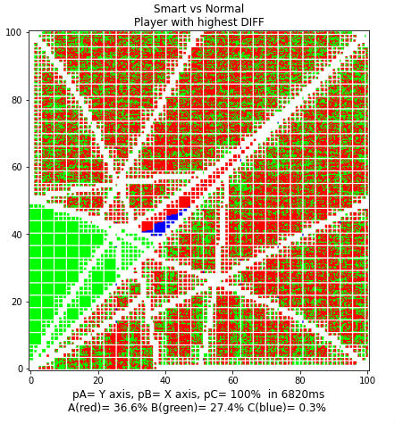 Truel solver as Python based Jupyter notebook